Example: Text Mining R

Initial Data Exploration

The next step is to get acquainted with the data set, and to get a feel for it. I always find this part especially exciting as this is for me new data, hence an exploratory process. Let’s take a look at the names of the variables (columns) and the type of each variable.

wine.data %>% 
  attr("spec")

## cols(
##   X1 = col_double(),
##   country = col_character(),
##   description = col_character(),
##   designation = col_character(),
##   points = col_double(),
##   price = col_double(),
##   province = col_character(),
##   region_1 = col_character(),
##   region_2 = col_character(),
##   taster_name = col_character(),
##   taster_twitter_handle = col_character(),
##   title = col_character(),
##   variety = col_character(),
##   winery = col_character()
## )

Above we can see that data set contains 14 variables, where only 3 of them are numeric, which is great when it comes to text mining. The variable that is of most interest for this example is the description variable, as it contains the longest passages of text. Moreover, the next thing I like to do is to clean the loaded data a little bit by renaming the X1 variable to index, as that is what it is.

wine.data <- wine.data %>% 
  rename(index = X1)

Tokenisation

Now, we can finally start exploring the data a bit deeper. A good practice is to visualise the data in order to facilitate the explorative process. Now, we are going to apply a process known as tokenization, which in short is the process of finding meaningful units of text, in this case, words that are of specific interest for us. Hence, tokenization is the processes of splitting up text into separate words, and because we are working in a tidy fashion, we are only going to have one word per observation (row).

# wine.data.per.word <- wine.data %>% 
#   unnest_tokens(word, 
#                 description)

wine.data.per.word %>% 
  names()

##  [1] "index"                 "country"              
##  [3] "designation"           "points"               
##  [5] "price"                 "province"             
##  [7] "region_1"              "region_2"             
##  [9] "taster_name"           "taster_twitter_handle"
## [11] "title"                 "variety"              
## [13] "winery"                "word"

During the tokenization process I also renamed one of the variables in order to ease the comprehension in an attempt to name it more appropiate I chose to rename the new variable “word”, which can be seen above. After the tokenization processes we now have a data set that contains 5334954 observations, whereas the data set only had 129971 observations from the start. A suitable next step is to remove what is known as stop words, that is words such as the, at and is. At this stage of the process these words are of no interest to us.

data("stop_words")

wine.data.per.word.no.stops <- wine.data.per.word %>% 
  anti_join(stop_words)

By removing the stop words we now have a data set with 2968316 observations, which means that almost half of the total word count was due to words that are not of interest to us. Now, we will count the occurrence of each word in order to explore if there are any words of interest.

wine.data.per.word.no.stops %>% 
  count(word, 
        sort = T) %>% 
  head(20)

## # A tibble: 20 x 2
##    word        n
##    <chr>   <int>
##  1 wine    78322
##  2 flavors 62791
##  3 fruit   49927
##  4 aromas  39639
##  5 palate  38437
##  6 acidity 34999
##  7 finish  34971
##  8 tannins 30877
##  9 drink   30318
## 10 cherry  29321
## 11 black   29020
## 12 ripe    27375
## 13 red     21782
## 14 spice   19233
## 15 notes   19045
## 16 oak     17758
## 17 fresh   17527
## 18 rich    17466
## 19 dry     17222
## 20 berry   16979

In the table above, the variable word contains the top 20 most frequently occurring words and n contains the number of occurrences. Because these texts are wine reviews, it is not surprising that words such as wine, flavours and drink are frequently occurring in the text, hence these words only provides limited additional insights and is there off of limited interest for us. Furthermore, through the word occurrence count it is possible to get a grasp of the distribution, where the maximum number of occurrences is 78322 and the minimum number is 1, with a mean of 90.49468. The mean tells us that there are some values that are extremely well used, whereas there are a wide variety of words, which is certainly confirmed by the number of different words, namely 32801 different words.

Sentiment Analysis

A suitable next step in this exploratory process would be to explore what is known as a sentiment analysis, in order to determine if the review is good or bad. We will start with a rudimentary sentiment analysis, just get the lay of the land so to speak. This rudimentary form of sentiment analysis is based upon looking at the sentiment of each word on its own, this is the most rudimentary form of sentiment analysis upon which one can dig deeper in order to better understand the context of the text.

We will use some well-established sentiment data set, which list words and their sentiments in different ways. We have 3 data sets at our disposal and each of them categorises words in their own way.

• AFINN, which lists word via a valency index spanning from -5 to 5. This data set is constructed by Finn Ã…rup Nielsen.
• bing, contains sentiments in form of positive or negative. This lexicon was created by Bing Liu and collaborators.
• nrc, attempts to put word into a more emotional context, and it was created by Saif Mohammad and Peter Turney.

We are going to start by using the bing lexicon in order to get a rough understanding of the distribution. Let us start by exploring the distribution of positive sentiments in relation to negative sentiments.

wine.data.per.word.no.stops %>% 
  inner_join(get_sentiments("bing")) %>% 
  count(sentiment, sort = T)

## # A tibble: 2 x 2
##   sentiment      n
##   <chr>      <int>
## 1 positive  348716
## 2 negative  107976

We can clearly see that there is a higher frequency of words with positive sentiments, roughly 3 times as many positive words.

Next, we will apply the AFINN lexicon in order to get a numeric scale instead. The reason for that is that it will be easier to test for possible correlations between the sentiment and other variables such as the rating of wine.

wine.data.per.word.no.stops %>% 
    inner_join(get_sentiments("afinn")) %>% 
    group_by(index, 
             title, 
             points) %>% 
  summarise(sum.score = sum(score)) %>% 
    ungroup() %>% 
    select(points, 
           sum.score) %>% 
  cor()

##              points sum.score
## points    1.0000000 0.2873469
## sum.score 0.2873469 1.0000000

As can be seen above there is a positive correlation between the summed up sentiments and the rating (points) of the wine. There are of course problems with this, the first is that a wine does not necessary have more words that are listed as positive just because they have a high ranking. The second problem is that a lot of words are left out due to the descriptive nature of wine reviews, where words like grapes, lemon, and soil is not in the lexicon but are very frequent in the reviews. But, let us investigate the first problem, that is whether there is a correlation between a higher word count of words with positive sentiments and a higher rating (points).

wine.data.per.word.no.stops %>% 
    inner_join(get_sentiments("afinn")) %>% 
    group_by(index, 
             title, 
             points) %>% 
  count(count.score = score > 0) %>% 
    ungroup() %>% 
    select(points, count.score) %>% cor()

##                points count.score
## points      1.0000000   0.0639772
## count.score 0.0639772   1.0000000

There seem to be a positive correlation, but very faint, which proves that the first assumption seem to be fallacious. With that out of the way we can move on to plot our first plot.

ggplot(
    wine.data.per.word.no.stops %>% 
        inner_join(get_sentiments("afinn")) %>% 
        group_by(index, 
                 title, 
                 points,
                 price) %>% 
        summarise(sum.score = sum(score)),
    aes(x = sum.score, y = points, colour = price)) + 
    geom_jitter()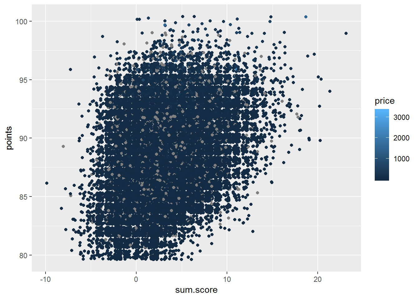

In the plot above we can see that we have the rating (points) of the wine on the y-axis and the total score from our sentiment analysis on the x-axis as well as price as colour, that is the lighter the colour the greater the price. There are some grey dots, which are observations where we lack information about the price. So let us remove the missing values and replot the plot.

ggplot(
    wine.data.per.word.no.stops %>% 
        inner_join(get_sentiments("afinn")) %>% 
        group_by(index, 
                 title, 
                 points,
                 price) %>% 
        summarise(sum.score = sum(score)) %>% 
      na.omit(),
    aes(x = sum.score, y = points, colour = price)) + 
    geom_jitter()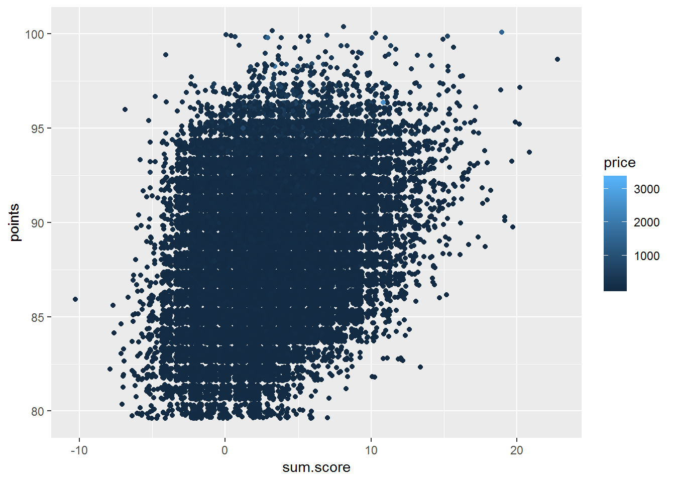

Now, when we have removed the missing values we can see that a lot of the wines with a high rating (points) tend to have a positive sentiment. The plot also shows us that the more expensive wines seem to be clustered around a high rating of 90 to 90 but only have a total sentiment score of 0 to 10.

It is easy to get carried away with digging for nuggets hidden in the data, in so forget why we are doing this from the start and that is to solve problems and provide value. So, what can the knowledge we have discovered thus far be used for. From a business perspective, we now have a way to position our self in a wine market, when it comes to both price and competitors. We can also explore which specific wines that each taster tend to have a preference towards and in so use that to ones advantage through sending a taster with a specific preference a product that he or she is more likely to give high points, that is good for marketing. Another example is from a more finance point of view, where the information about the tastes can be applied to create a portfolio that optimises the return and minimises the risk.